Sewing Chiral RCFTs

Given a local RCFT defined on a punctured sphere ${𝕊}^2\left(\left\{{𝑝}_1,{𝑧}_1\right\},\dots ,\left\{{𝑝}_{𝑛},{𝑧}_{𝑛}\right\}\right)$, we want to construct such a theory on a higher genus Riemann surface ${\mathrm{\Sigma }}_{𝑔}\left(\left\{{𝑝}_1,{𝑧}_1\right\},\dots ,\left\{{𝑝}_{𝑛},{𝑧}_{𝑛}\right\}\right)$, where $\left\{{𝑝}_{𝑛},{𝑧}_{𝑛}\right\}$ denotes the puncture at point ${𝑝}_{𝑛}$ with local coordinate ${𝑧}_{𝑛}$, which satisfies $𝑧\left(𝑝\right)=0$.

There is a standard way to obtain a higher genus Riemann surface from some punctured spheres, so-called factorization, or sewing procedure. Thus, the main idea is:

• First, find a factorization of the target Riemann surface ${\mathrm{\Sigma }}_{𝑔}\left(\left\{{𝑝}_1,{𝑧}_1\right\},\dots ,\left\{{𝑝}_{𝑛},{𝑧}_{𝑛}\right\}\right)$.
• Define local RCFTs on each of the pants, i.e. ${𝕊}^2\left(\left\{{𝑝}_{𝑖},{𝑧}_{𝑖}\right\},\left\{{𝑝}_{𝑗},{𝑧}_{𝑗}\right\},\left\{{𝑝}_{𝑘},{𝑧}_{𝑘}\right\}\right)$.
• Find an associative sewing operation for local RCFTs, which is compatible with the sewing of Riemann surfaces.

The data above could be summarized as:

where $𝑍$ denotes the RCFT defined on the corresponding Riemann surface, corresponding to the higher genus partition functions.

Since there are various factorizations for a given Riemann surface, we also need to show that the final RCFT defined on ${\mathrm{\Sigma }}_{𝑔}\left(\left\{{𝑝}_1,{𝑧}_1\right\},\dots ,\left\{{𝑝}_{𝑛},{𝑧}_{𝑛}\right\}\right)$ is independent of the choice of pants decomposition. Which could be related to the constrains for $𝑍$ above, corresponding to the Moore-Seiberg data in the rational CFT and mapping class group actions on the Riemann surfaces.

Introduction: Gluing in QFT

This is an elementary part which is well-known in QFT at least in the level of “philosophy”.

Consider a QFT defined on a manifold $𝑀$ with boundary $𝜕𝑀$, the path integral could be written as:

which is a functional of the boundary field configuration $𝜑\left(𝜕𝑀\right)$. Thus, if we have two manifolds $𝑀$ and $𝑁$ with isomorphic boundaries $𝜕𝑀\equiv 𝜕𝑁$, we could glue them together to form a new manifold $𝑀{\bigsqcup }_{𝜕𝑀\equiv 𝜕𝑁}𝑁$ with inverse boundary operations:

where we sum over all the possible boundary field configurations $𝜑\left(𝜕𝑀\right)$, and $𝑍\left(𝑁,𝜑\left(𝜕𝑀\right)\right)$ denotes the complex conjugate of $𝑍\left(𝑁,𝜑\left(𝜕𝑀\right)\right)$, since the orientation of $𝜕𝑁$ is opposite to that of $𝜕𝑀$.

Sewing an RCFT

We first review the sewing procedure for Riemann surfaces, then discuss how local RCFTs behave under such operations.

Sewing Riemann Surfaces

Consider two punctures $\left\{{𝑝}_{𝑖},{𝑧}_{𝑖}\right\}$ and $\left\{{𝑝}_{𝑗},{𝑧}_{𝑗}\right\}$ on (some) Riemann surfaces. A sewing operation would glue these two punctures together to form a new Riemann surface ${\mathrm{\Sigma }}^{\prime }$.

In this procedure:

• Punctures ${𝑝}_{𝑖}$ and ${𝑝}_{𝑗}$ would be identified and finally removed.
• The local coordinates ${𝑧}_{𝑖}$ and ${𝑧}_{𝑗}$ would satisfy the relation ${𝑧}_{𝑖}{𝑧}_{𝑗}=𝑞$, where $𝑞$ is a complex parameter with $|𝑞|<1$.

The second step could be understood as follows:

• Cutting out small disks $|{𝑧}_{𝑖}|<|𝑞{|}^{\frac{1}{2}}$ and $|{𝑧}_{𝑗}|<|𝑞{|}^{\frac{1}{2}}$ around the punctures.
• Identifying the boundary $|𝑞{|}^{\frac{1}{2}}\le |{𝑧}_{𝑖}|<1$ and $|𝑞{|}^{\frac{1}{2}}\le |{𝑧}_{𝑗}|<1$ via the relation ${𝑧}_{𝑖}{𝑧}_{𝑗}=𝑞$.

Modularity and Mapping Class Group

A Fenchel–Nielsen coordinate system $\left\{{𝑞}_{𝑖}\right\}$ corresponds to a factorization of the Riemann surface. However, there are various factorizations for a given Riemann surface, thus various coordinate systems $\left\{{𝑞}_{𝑖}\right\}$ in the Teichmüller space.

Modularity: Sewing a Double Punctured Sphere

Consider sewing two punctures $𝑝$ and $𝑞$ on a double punctured sphere ${𝕊}^2\left(\left\{𝑝,𝑧\right\},\left\{{𝑝}^{\prime },𝑤\right\}\right)$, the resulting Riemann surface is a torus (well-known fact). We assume $𝑝$ and ${𝑝}^{\prime }$ are two poles of the sphere, and the local coordinates $𝑧$ and $𝑤$ are related by $𝑧𝑤=𝑞$.

Using the transition function of two charts on the sphere, we could write $𝑤=\frac{1}{𝑧}$, thus the sewing relation could be written as and identification $𝑧\sim 𝑞𝑧$. Under this identification, the complex plane $ℂ$ becomes a torus $𝕋={ℂ}^{\ast }/\left(𝑧\sim 𝑞𝑧\right)\cong ℂ/\left(\mathbb{Z}+𝜏\mathbb{Z}\right)$, where $𝑞={𝑒}^{2𝜋𝑖𝜏}$, $𝜏\in ℍ$.

The change of sewing could be identified with changing the way to cut the torus into a double punctured sphere, which is identified with changing the basis of the homology group ${𝐻}_1\left(𝕋,\mathbb{Z}\right)$ (A-cycle and B-cycle). The homology basis has a natural symplectic structure given by the intersection number, thus the change of basis should preserve such structure, i.e., an action of the symplectic group $\text{Sp}\left(2,\mathbb{Z}\right)\equiv \text{SL}\left(2,\mathbb{Z}\right)$.

Thus, the different sewing operations on the double punctured sphere correspond to different coordinate systems $𝑞={𝑒}^{2𝜋𝑖𝜏}$ and ${𝑞}^{\prime }={𝑒}^{2𝜋𝑖{𝜏}^{\prime }}$ on the Teichmüller space of the torus, which are related by the modular group $\text{SL}\left(2,\mathbb{Z}\right)$ action.

Mapping Class Group

Higher dimensional generalization of the modular group is the mapping class group of Riemann surfaces. Point is: Different sewing operations correspond to the different $\left\{{𝑞}_{𝑖}\right\}$ coordinate systems in the Teichmüller space, which are related by the action of the mapping class group ${\text{MCG}}_{𝑔,𝑛}$, which is $\text{SL}\left(2,\mathbb{Z}\right)$ in the torus case.

Elementary Moves for Sewing Operations

A sewing procedure could be decomposed into a sequence of elementary sewing operations, which correspond to:

• Self twisting ${\mathrm{\Sigma }}_{𝑔,𝑛}^{\prime }={𝑇}^{𝑖}{\mathrm{\Sigma }}_{𝑔,𝑛}$.
• Self sewing ${\mathrm{\Sigma }}_{𝑔+1,𝑛-2}^{\prime }=8_{𝑗}^{𝑖}{\mathrm{\Sigma }}_{𝑔,𝑛}$.
• Sewing two different Riemann surfaces ${\mathrm{\Sigma }}_{{𝑔}_1+{𝑔}_2,{𝑛}_1+{𝑛}_2-2}^{\prime }={\mathrm{\Sigma }}_{{𝑔}_1,{𝑛}_1}{\infty }_{𝑗}^{𝑖}{\mathrm{\Sigma }}_{{𝑔}_2,{𝑛}_2}$.

And the resulting Riemann surface could be obtained by a sequence of compositions of these elementary sewing.

There are various ways to go from a given factorization to another one, which correspond to different sequences of elementary sewing operations. There is a result by Hatcher and Thurston that classifies these relations:

Thus, to obtain two consistent sewing operations from a given factorization to another one, we only need to check the consistency under these elementary moves. The relations such as pentagon relation and hexagon relation shows that, all the different ways to go from a given factorization to another one are consistent.

Sewing Local RCFTs

Using the construction above, the theory has a strong flavor of our naive picture of path integral gluing in QFT, i.e., summing over the states living on the boundary circles:

where ${𝜑}_{𝛼}$ denotes the boundary local field configurations. In CFT:

• Using state-field correspondence, the boundary local field configurations are identified with the states in the Hilbert space $𝐻$ attached to the boundary circle.

• Boundary field configurations could be written as linear combinations of primary fields and their descendants:

  $${\mathrm{ℒ︀}}_{-𝑛}{𝜑}_{𝑖}\left(𝑧\right)≔{𝐿}_{-{𝑛}_1}\dots {𝐿}_{-{𝑛}_{𝑁}}{𝜑}_{𝑖}\left(𝑧\right),$$
  where $\left\{{𝜑}_{𝑖}\right\}$ is the set of primary fields, and $\left\{{𝐿}_{𝑛}\right\}$ are the Virasoro generators (we only consider chiral part here for simplicity).
• RCFT restricts the dimensional of the Hilbert space $𝐻$ to be finite, thus we could select a finite basis $\left\{{𝜑}_{𝑖}\right\}$ for the primary fields.

Thus, we could select a finite basis for the states living on the boundary circles $\left\{|𝑖,𝑛⟩\right\}$, where $𝑖$ labels the primary fields, and $𝑛$ labels the descendants. Consider sewing $𝑀$ with puncture $𝑝$ and $𝑁$ with puncture $𝑞$, the boundary state could be written as:

where the coefficients ${𝐴}_{𝑖,𝑛}$ and ${𝐵}_{𝑗,𝑚}$ could be written as some correlation functions involving the corresponding fields:

where we used state-operator correspondence to relate the states and local fields, here the puncture is understood as infinite past or future in the radial quantization.

The gluing procedure leads to a two punctured sphere, whose end points are inserted with the boundary states generated by descendants of primary fields. Thus, the partition function on such sphere ${𝕊}^2\left(\left\{𝑝,𝑧\right\},\left\{𝑞,𝑤\right\}\right)$ is¹:

thus, the amplitude from sewing $𝑀$ and $𝑁$ could be written as:

(here we assume that $𝑀$ is positive definite). Inserting this into the correlation functions on $𝑀$ and $𝑁$, we obtain the sewn chiral correlation function:

Now we focus on the primary fields correlator. Due to the state-operator correspondence, a primary field would correspond to a highest weight state, thus form a subspace in the Hilbert space ${𝑉}_{ℎ}$. In this case, the setup for our sewing operation could be summarized as:

• Consider sewing two Riemann surfaces $𝑀$ and $𝑁$ at punctures $𝑝$ and $𝑞$.
• On each puncture, we attach a vector space ${𝑉}_{ℎ}$ spanned by the primary field ${𝜑}_{ℎ}$ and its descendants.

The second part corresponds to choosing a module ${𝑉}_{ℎ}$ of our chiral algebra $𝑉$ (or vertex operator algebra if you like) to attach to the sewing punctures.

Reviewing our previous discussion, we have:

We need to check that the conformal blocks constructed above indeed form a basis of the space of conformal blocks $\mathrm{ℬ︀}\left({𝑉}_{{ℎ}_1},\dots ,{𝑉}_{{ℎ}_{𝑛}}\right)$. We will do this in the next section.

An-Aside: Three Point Sphere Conformal Blocks and Intertwining Operators

The conformal blocks on three point sphere ${𝕊}^2\left(\left\{{𝑝}_1,{𝑧}_1\right\},\left\{{𝑝}_2,{𝑧}_2\right\},\left\{{𝑝}_3,{𝑧}_3\right\}\right)$ is related to the fusion rules of the modules attached to the punctures:

which lead us to consider the intertwining operators among the modules:

where ${\mathrm{\Phi }}_{𝑗,𝑘}^{𝑖}\left(𝑧\right)$ have conformal weight ${ℎ}_{𝑖}$, mapping (intertwining) the module ${𝑉}_{{ℎ}_{𝑗}}$ to ${𝑉}_{{ℎ}_{𝑘}}$. If there are various intertwining operators of the same type, we denote them by ${\mathrm{\Phi }}_{𝑗𝑘}^{𝑖,𝛼}\left(𝑧\right)$ where $𝛼=1,\dots ,{𝑁}_{𝑖𝑗}^{𝑘}$, thus the three point sphere conformal blocks could be written as:

In the language of intertwining operators, the sewing operation which leads to the four point sphere conformal blocks $\mathrm{ℬ︀}\left({𝑉}_{{ℎ}_{𝑖}},{𝑉}_{{ℎ}_{𝑗}},{𝑉}_{{ℎ}_{𝑘}},{𝑉}_{{ℎ}_{𝑙}}\right)$ could be written as:

where ${𝑉}_{𝑝}$ is the internal module attached to the sewing puncture, and the factorization above corresponds to the s-channel Feynman diagram $\left(𝑖𝑗\right)𝑘\to 𝑙$.

Consistency Conditions

At the previous section, we have defined a sewing operation for local RCFTs, which is associated with the sewing of Riemann surfaces, and the gluing procedure in QFT.

However, such a construction is just “a” construction, to make it become “a consistent” construction of higher genus RCFTs from lower genus ones, we need to check some consistency conditions:

• Check the RCFT chiral correlator we defined is indeed a chiral correlator.
• There are various factorizations for a given Riemann surface, we need to show that the final RCFT defined is independent of the choice of pants decomposition.
• There are various way from a given factorization to another one, we need to check the consistency of these different ways.

The first point is the inner constrain for RCFT itself, where we have already mentioned it before, and second point is the outer constrain from the geometry of Riemann surfaces, corresponding to the mapping class group actions.

Different Sewing Operations:

Gives Same Theory

A physical field theory defined on a Riemann surface should be independent of the choice of factorization of the surface, thus independent of the choice of sewing operations.

Recall our previous construction of conformal block basis from a given factorization, different factorizations would give different bases of the space of conformal blocks $\mathrm{ℬ︀}\left({𝑉}_{{ℎ}_1},\dots ,{𝑉}_{{ℎ}_{𝑛}}\right)$. What we need is to show that these different bases actually span the same space.

Thus, different factorizations give different bases of the same space of conformal blocks $\mathrm{ℬ︀}\left({𝑉}_{{ℎ}_1},\dots ,{𝑉}_{{ℎ}_{𝑛}}\right)$. Which shows that our sewing operation for local RCFTs is consistent with the geometry of Riemann surfaces.

Consistent under Sewing Parameter Change: Elementary Moves

While different factorizations give rise to different bases of the space of conformal blocks, the change of basis must be independent of the chosen sequence of elementary sewing operations.

Like what we have mentioned before, to check such consistency, we only need to check the elementary moves given by Hatcher-Thurston theorem, i.e., F-move and S-move.

Such move would lead to a change of basis of the space of conformal blocks, we denote such change of basis by some matrices.

F-Move

F-move corresponds to changing the way to cut a four punctured sphere into two three punctured spheres, i.e., consider ${𝕊}^2\left({𝑝}_{𝑖},{𝑝}_{𝑗},{𝑝}_{𝑘},{𝑝}_{𝑙}\right)$, F-move would correspond to exchanging $\left(𝑙𝑘\right)𝑗\stackrel{𝑝}{\to }𝑖$ and $𝑙\left(𝑗𝑘\right)\stackrel{𝑞}{\to }𝑙$ channel. Here, $𝑝$ $𝑞$ denote the internal modules attached to the sewing punctures.

Thus, F-move would lead to a change of basis of the space of four-point conformal blocks, i.e. ${\left\{{\mathrm{\Phi }}_{𝑖𝑝}^{𝑗}{\mathrm{\Phi }}_{𝑝𝑙}^{𝑘}\right\}}_{𝑝}$ and ${\left\{{\mathrm{\Phi }}_{𝑗𝑞}^{𝑘}{\mathrm{\Phi }}_{𝑖𝑙}^{𝑞}\right\}}_{𝑞}$, which could be written as:

where the matrix ${𝐹}_{𝑝𝑞}\left[\begin{array}{cc}𝑗& 𝑘\\ 𝑖& 𝑙\end{array}\right]:{𝑉}_{𝑞𝑙}^{𝑖}\otimes {𝑉}_{𝑗𝑘}^{𝑞}\to {𝑉}_{𝑗𝑝}^{𝑖}\otimes {𝑉}_{𝑘𝑙}^{𝑝}$ is called the F-matrix, and column $\left[𝑗,𝑘\right]$ denotes the fusion of modules ${𝑉}_{{ℎ}_{𝑗}}$ and ${𝑉}_{{ℎ}_{𝑘}}$, and row $\left[𝑖,𝑙\right]$ denotes the initial modules ${𝑉}_{{ℎ}_{𝑖}}$ and outer module ${𝑉}_{{ℎ}_{𝑙}}$.

S-Move

The S-move corresponds to changing the way to cut a one punctured torus into a double punctured sphere, i.e., consider ${𝕋}^2\left(\left\{𝑝,𝑧\right\}\right)$, S-move would correspond to exchanging the A-cycle and B-cycle cutting.

We assume the puncture $𝑝$ is attached with module ${𝑉}_{{ℎ}_{𝑖}}$.

The A-cycle cutting corresponds to cutting the torus into a double punctured sphere ${𝕊}^2\left(\left\{𝑝,𝑧\right\},\left\{𝑞,𝑤\right\}\right)$, where the punctures $𝑝$ and $𝑞$ are attached with modules ${𝑉}_{{ℎ}_{𝑗}}$ and ${𝑉}_{{ℎ}_{{𝑗}^{\vee }}}$ respectively. Thus, the intertwining operator could be written as ${\mathrm{\Phi }}_{𝑗𝑗}^{𝑖}\left(𝑧\right)$, and the conformal block space could be written as:

And the partition function on the torus could be written as:

where $𝛽$ (a primary state) denotes the boundary filed configuration at the puncture $𝑝$.

The B-cycle cutting corresponds to cutting the torus into a double punctured sphere ${𝕊}^2\left(\left\{𝑝,𝑧\right\},\left\{{𝑞}^{\prime },𝑤\right\}\right)$, where the punctures $𝑝$ and ${𝑞}^{\prime }$ are attached with modules ${𝑉}_{{ℎ}_{𝑘}}$ and ${𝑉}_{{ℎ}_{{𝑘}^{\vee }}}$ respectively.

Thus, though the cutting are different, both of them give a basis of the same space of conformal blocks ${\mathrm{ℬ︀}}_{1,1}\left({𝑉}_{{ℎ}_{𝑖}}\right)≔{⨁}_{𝑗\in \mathrm{𝒥︀}}{𝑉}_{𝑖𝑗}^{𝑖}$, thus the only difference is the change of basis, which could be written as:

Braiding Move

Unlike the punctured space case, conformal blocks on Riemann surfaces carries some important analytical structure, which leads to some nontrivial monodromy, and thus braiding operations.

The braiding move corresponds to exchanging two punctures on the Riemann surface, which leads to a map:

The full correlator function should be invariant under such braiding operation, thus the chiral part should transform linearly under such operation:

where the matrix ${𝐵}_{𝑝𝑞}\left[\begin{array}{cc}𝑗& 𝑘\\ 𝑖& 𝑙\end{array}\right]:{𝑉}_{𝑗𝑝}^{𝑖}\otimes {𝑉}_{𝑘𝑙}^{𝑝}\to {𝑉}_{𝑗𝑞}^{𝑖}\otimes {𝑉}_{𝑘𝑙}^{𝑞}$ is called the braiding matrix.

Twisting Move

The twisting move corresponds to twisting a puncture on the Riemann surface by $2𝜋$ (Dehn twist), which leads to a map:

Consistent under Sewing Parameter Change: Moore-Seiberg Equations

We have discussed the elementary moves (F and S move) leading to different sewing operations, which give rise to linear transformations $\left(𝐹,𝑆,𝐵,𝑇\right)$ on the space of conformal blocks.

Now we need to check the consistency of these transformations.

Firstly, as we mentioned before, different sequences of elementary moves from a given factorization to another one should give the same transformation on the space of conformal blocks.

Moreover, since we attach some RCFT data on these Riemann surfaces, these transformations should be compatible with the RCFT data. Thus, our consistency conditions could be summarized as:

• Consistency of local RCFT data.
• Monodromy of conformal blocks form representations of the mapping class group.
• Different paths of the elementary moves relate same basis of conformal blocks.

Such consistency conditions are called the Moore-Seiberg equations, or Duality identities.

On genus zero Riemann surfaces, we have the following Moore-Seiberg equations:

• Pentagon relation for the F-move.
• Hexagon relation for the B-move and F-move.

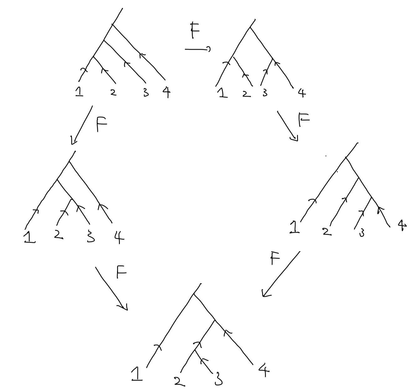
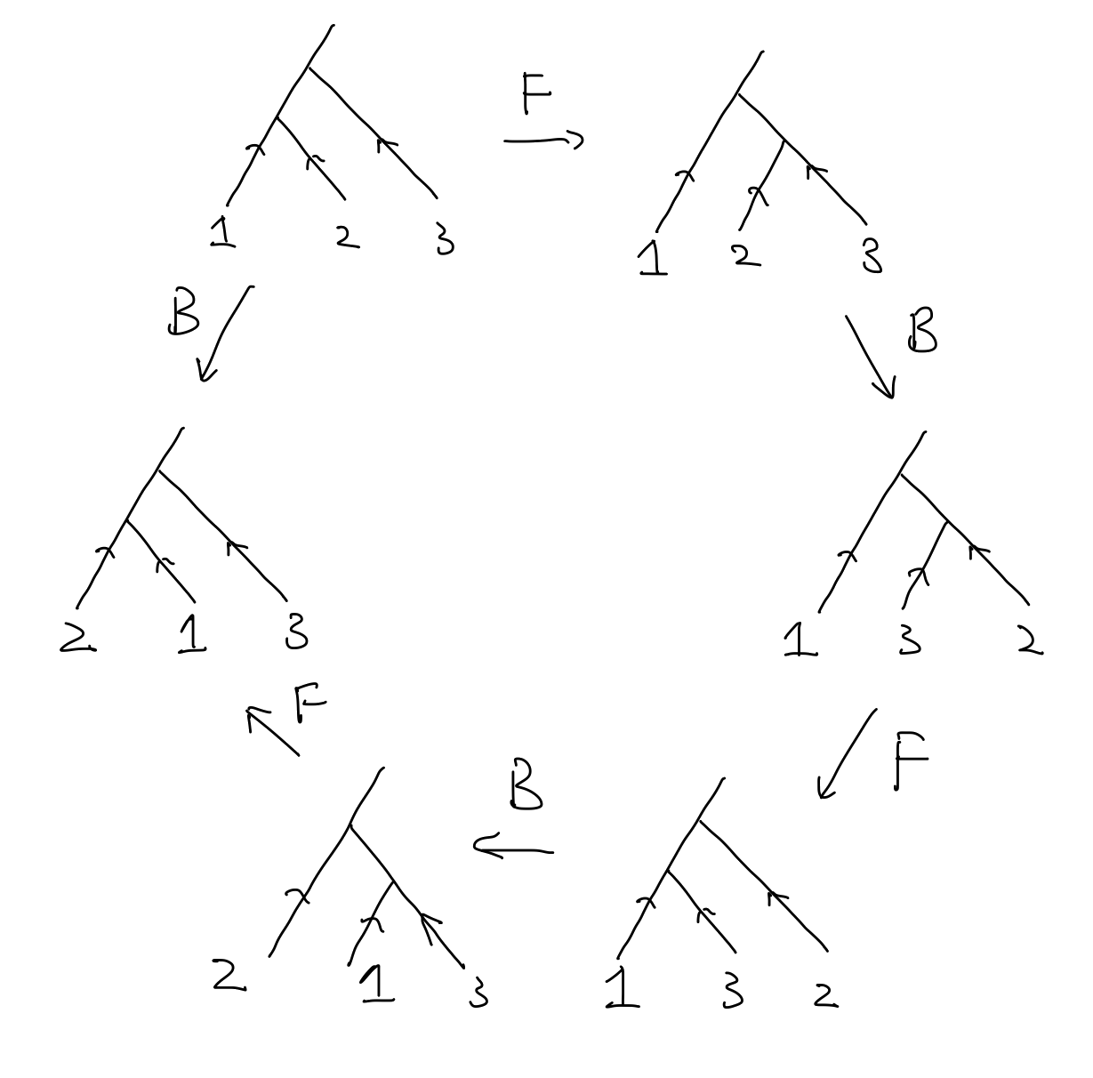
From these relations, $𝐵$ satisfies the Yang-Baxter equation.

Moreover, we have some modularity conditions for the S-move on genus one Riemann surfaces:

• ${𝑆}^2\left(𝑗\right)=\pm 𝐶{𝑒}^{𝑖𝜋{ℎ}_{𝑗}}$, where $𝐶$ is the charge conjugation matrix.
• ${\left(𝑆𝑇\right)}^3={𝑆}^2$ and some other relations coming from the modular group $\text{SL}\left(2,\mathbb{Z}\right)$.
• Other genus one relations, e.g., $𝑆𝑎{𝑆}^{-1}=𝑏$.

You may wander would there be some higher genus Moore-Seiberg equations? The answer is yes, however, as we will see in the next section, all these higher genus consistency conditions could be derived from the genus zero and one Moore-Seiberg equations, i.e., the independent consistency conditions are just these we mentioned above.

Completeness of the Consistency Conditions

It seems that we can construct infinitely many consistency conditions from various sewing operations on Riemann surfaces.

However, there is a result by Moore and Seiberg that shows that all these consistency conditions could be derived from a finite set of them, i.e., the Moore-Seiberg equations we mentioned before.

Abstract Nonsense Explanation

The simplest way to see this is using some “abstract nonsense” from category theory.

Note that the data $\left(𝐹,𝑆,𝐵,𝑇\right)$ we discussed above actually form a tensor category, or more precisely, a modular tensor category, using the MacLane’s coherence theorem, such finite set of consistency conditions could be understood as the coherence conditions for the modular tensor category, thus all the other consistency conditions could be derived from them, i.e., the diagrams constructed from these data commute.

Geometric Explanation: Mapping Class Group Representations

However, the geometric meaning of such consistency might be more “physical”, and related to the mapping class group actions on the Riemann surfaces.

The sewing procedures and the translations between them could be captured by a complex so-called the duality complex, where:

• Vertices: A basis of conformal blocks space.
• Edges: An elementary move ($𝐹$, $𝐵$, $𝑇$, $𝑆$ matrix) between two factorizations.

What we want to prove is that, all the loops in such complex are contractible while Moore-Seiberg equations are satisfied.

First, the pentagon relation of $𝐹$ matrix can be used to transform any vertex to a standard form, called the Multiperipheral Basis.

Now, the only remaining edges are related to $𝐵$, $𝑇$, and $𝑆$ moves. Thus, such operations could be identified with the elements of the mapping class group ${\text{MCG}}_{𝑔,𝑛}$.

Using this fact, every large loop in the duality complex could be decomposed into a sequence of smaller loops, each of which corresponds to a relation in the mapping class group:

• Braiding loop, which is contactable due to the hexagon relation of $𝐵$ and $𝐹$ matrix (Yang-Baxter equation).
• Dehn twist relations, which is contractible due to the modularity relations of $𝑆$ and $𝑇$ matrix.

Thus, all the loops in the duality complex are contractible while the Moore-Seiberg equations are satisfied.

1. ¹Here we assume $𝑞=1$ for simplicity, if we consider general sewing parameter $𝑞$, we need to insert an additional factor ${𝑞}^{{𝐿}_0-\frac{𝑐}{24}}$ to take care of the change of complex structure.